

Quantitative cyber risk measurement is more than guessing. It’s akin to estimating, or using what’s known along with the psychology of cyber threats to determine the probability of what is likely to happen. But there’s plenty to be done using data science and statistical analysis to “re-educate the guess.”
In this article we’ll look at some models and methods for improving estimation when calculating risk in the financial gamble of investing in cybersecurity defense.
What’s the Point?
The science of analytics can be a powerful tool in extracting insight from an otherwise meaningless mass of data. Think about the conclusions that can be made based on weeks or months of stock market data versus just one day—time-based trends and distribution curves can reveal things otherwise obscured at a narrow glance.
The business of information technology, and cybersecurity specifically, requires leaders and managers to make judgment calls for everything from resource allocation to budgeting in constant refinement of a strategy and defensive posture. How to task expensive analyst or incident response talent is often a reactive, event-based decision, but longer term cost planning like tooling or service subscriptions might require a little more thought to determine the potential return on investment.
What if we could run some numbers to make the most accurate decision based on known past events? What if our guess doesn’t have to be a swing in the dark? We’re usually sitting on mountains of data from our own tools as well as what’s available on the Internet, so let’s use them to make more scientific decisions, or best guesses, in security.
What Is Risk?
Anytime we’re exposed to a potential undesirable consequence, or don’t know the outcome of an uncertain scenario, whether in cybersecurity or in life, it’s called risk. For example:
- Will you suffer a data breach?
- When will the next phishing email arrive?
- When will a cyberattack on my organization happen?
It’s not possible to know the answers to these questions. Risk is a term that’s often used to quantify the likelihood of a negative event. It’s about uncertainty.
Quantifying Risk
The question is: how do you quantify something if the future state of it is unknown, then translate it into business metrics your CISO and other stakeholders or decision makers can understand? You’re not alone. Most people tasked with implementing security programs struggle with this.
If risk means we don’t know what will happen in the future, then when we quantify it, the reality is we’re guessing.
Is guessing okay? Does it help you understand your environment better and better justify your need for a budget or additional resources?
It is okay to guess. And there’s a methodology to making guesses better. If you are basing your guesses on knowledge you have combined with psychology, you can better estimate what will happen in the future, even if you’re uncertain.
What You’re Doing Wrong
Below is a relatively standard risk matrix, and many are probably already familiar with it or use it in their organizations. It lets you rate things on scale of 1-5; low, medium, and high; or reds and greens to assess which risks exist for different vulnerabilities. Or, just overall risk.
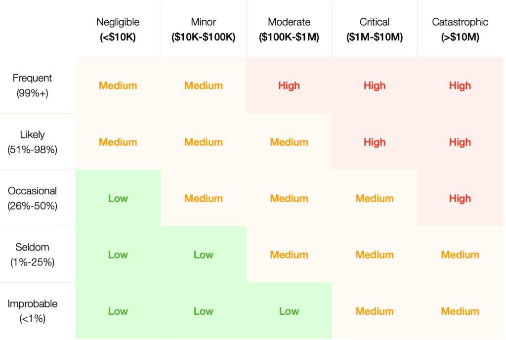
The matrix above is a model that leverages arbitrary, non-quantitative scales, compressed ranges, and introduces uncertainty into estimates. What this means is that a 1, on a scale of 1-5, is actually an uncertain measurement, especially with ranges that are dimensionless and subjective by their very nature.
The problem with introducing these abstract scales and methods is not only the uncertainty they introduce, but that they provide the worst possible understanding of the risks we are trying to analyze.
Such arbitrary representations can result in something called the Analysis Placebo, an outcome that occurs when data is analyzed using statistically or mathematically incorrect models. It results in something worse than nothing at all: no measurable gain in understanding. It applies not only to cybersecurity but any type of data analysis.
How Do We Get Better at Guessing?
Most people are bad at guessing. Statistically, this is because they are either over-confident or under-confident.
One method of improving guesses relies on using confidence intervals: a range of values within which we are fairly certain the correct answer lies. The correct value can be determined by using background knowledge and a bit of psychology.
Example: you may not know if your company will be hit by a phishing attack tomorrow, but you know how many attacks you had last year and you know how many people clicked the link the phishing training email.
That means you have some data, but you don’t know for sure.
The Equivalent Bet Method
The Equivalent Bet Method is a mental aid that helps people give better estimates and could be used to estimate cybersecurity risk more accurately by quelling the overconfidence effect. When someone is overconfident in means their estimates are wrong more often than they think.
The tool was developed by Carl Spetzler and Carl-Axel Von Holstein and reintroduced by Doug Hubbard in his book How to Measure Anything in 2007. It’s a simple tool for eliminating biases in judgement caused by over and under-confidence.
To use it simply introduce the topic, add a monetary risk (any amount that would incentivize winning over losing). Present three choices and ask players to estimate their 90% confidence interval answer.
The idea is to determine if they are truly 90% confident about the estimate. Perhaps use actual security tools currently in use to help analysts learn to make better estimates.
The Monte Carlo Simulation
The Monte Carlo simulation uses the data from the same input sources as risk matrixes where scales (1-5) are used to estimate. Why? Because it is a statistical model that accounts for uncertainty.
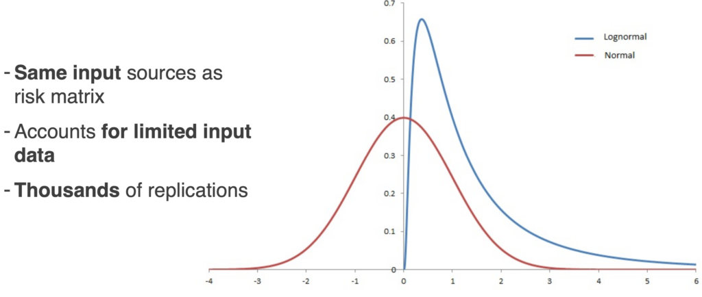
It accounts for uncertainty by using those ranges of 90% confidence intervals as inputs. It then runs thousands of replications against different scenarios which results in an average in terms of cost and risk. To do this it uses an underlying distribution.
In this example the Lognormal distribution is used. It’s a good one to use for cybersecurity assessments because most of the curve density is close to zero. It also doesn’t go below zero.
Getting the Input Data
There are a few steps in defining and refining input data to run the Monte Carlo simulations.
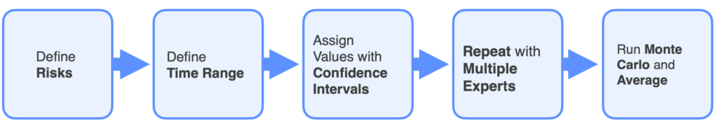
1 Define the risks
- What is being modeled?
- What is the risk you’re trying to determine?
- How risky are you?
Then translate this into cost.
2 Define the time range for the risk
Adding constraints to the time period under consideration is necessary because input data is associated with, and only accurate for events relative to trailing or leading time.
3 Assign values to the input variables
Do this using the confidence intervals explained earlier. If you happen to be working without historical data, you’ll need to interview your subject matter experts to get appropriate sample data.
Calibrate the confidence intervals using techniques like the Equivalent Bet method. It will help ensure you’re getting their true 90% confidence intervals and that they get a better understanding of their uncertainties.
Repeating the process with multiple experts is and averaging the results is a good way to achieve better real-world accuracy.
Use these to run Monte Carlo simulations. Values will evolve over thousands of replications using them on the underlying distribution, then you’ll take some averages.
Running Monte Carlo Simulations
There are other ways of doing this, but using Microsoft Excel is the easiest, and can generate a simple model quickly.
| Input Variables | Lower Bound | Upper Bound |
|---|---|---|
| Likelihood of experiencing a successful phishing attack in the next 12 months | 45% | 80% |
| Likelihood of a data breach resulting from a successful phising attack | 40% | 70% |
| Business impact of a data breach | $ 50,000.00 | $ 3,000,000.00 |
| Number of users that click on a phish in 12 month period | 500 | 2500 |
| Likelihood of users requiring response, remediation, and recovery | 2% | 5% |
| Hours to respond, remediate, and recover | 1 | 2 |
| Hourly wage of person remediating | $ 15.00 | $ 30.00 |
| % of user productivity truly lost during time to respond, remidiate, and recover | 75% | 90% |
| Estimated reduction in sucessful phising attacks with Phishing Detection and Response software | 80% | 90% |
| Cost of control Area 1, Cofense, Proofpoint, Ironscales (start with proofpoint and ironscales) | $ 15,000.00 | $ 50,000.00 |
| Cost to implement control | $ 5,000.00 | $ 25,000.00 |
This example profiles a fictitious company considering a purchase of cloud security products or services.
The input variables include company-specific data such as annual public configurations changes, possible misconfigurations, possible breaches caused by a misconfiguration, and add breach costs that can be pulled from reports such as the Verizon Data Breach Report or the IBM Costs of a Data Breach report, among other resources.
It includes costs of purchasing and implementing Cloud Security Posture Management (CSPM). Each input variable assumes the positive outcome of the previous, using conditional probability. The last input is the estimated reduction in misconfigurations after the purchase and implementation of a CSPM.
How Do the Input Variables Relate to Each Other?
This step is essential in formulating the equation to simulate. Consider the relationship of the first two variables, the number of times a public configuration changes along with the likelihood of a single change containing a misconfiguration, these two will be multiplied in the end equation.
Once the entire equation is mapped out and all variables related to each other, the simulation is ready to run.
Any number of replications can be used, but in this example 10,000 replications are run against the Lognormal distribution because it’s a middle number that falls between processing power and statistical averaging.
The simulation generates 10,000 different dollar amounts since it represents 10,000 different scenarios of all the input variables. An average of results can then be taken to find a simple value.
The first thing a company estimating the risk vs cost might look at is the average total annual cost of not purchasing and implementing the tool of service under evaluation. Compare that against the average cost of buying and implementing it, and finally the estimated return on investment (ROI). In the example shown, the ROI was 2.7 which would indicate that the company should buy and implement the tool/service as it would be saving more than it would spend.
All this effort is to reduce the decision making to a level playing field. When it can be broken down to dollars and ROI, that’s what should be presented to the board and CEO. The process has reduced the noise and complexity of their decision.
Simulated Loss Histogram and Loss Exceedance Curves
One of the other cool things you can get from the simulations is the Simulated Loss Histogram.
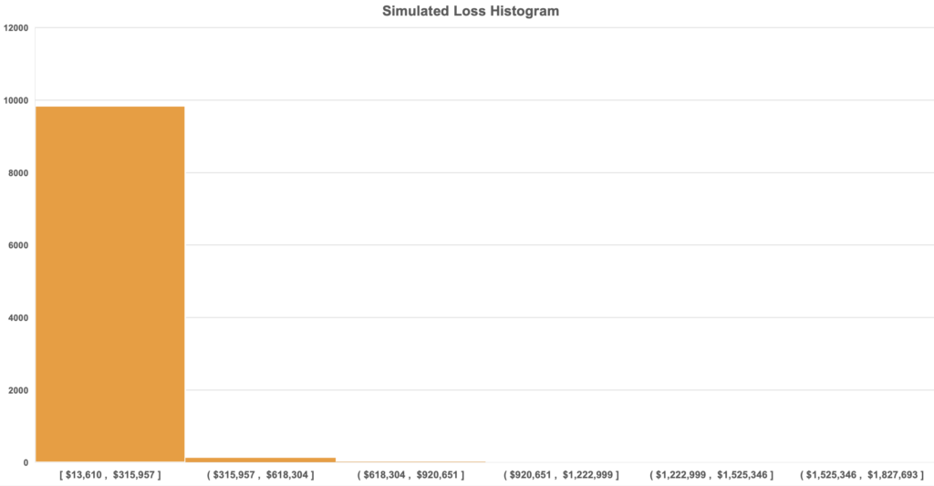
The above bar graph has one big, prominent bar because in most cases a data breach won’t be of the multi-million dollar variety, but a smaller, modest amount. Most of the simulations, over 9,900 of them, are reflected in the first bar.
Higher cost ones are included because you do need to account for the possibility even though they are less likely to happen.
Another product of the simulations are Loss Exceedance Curves.
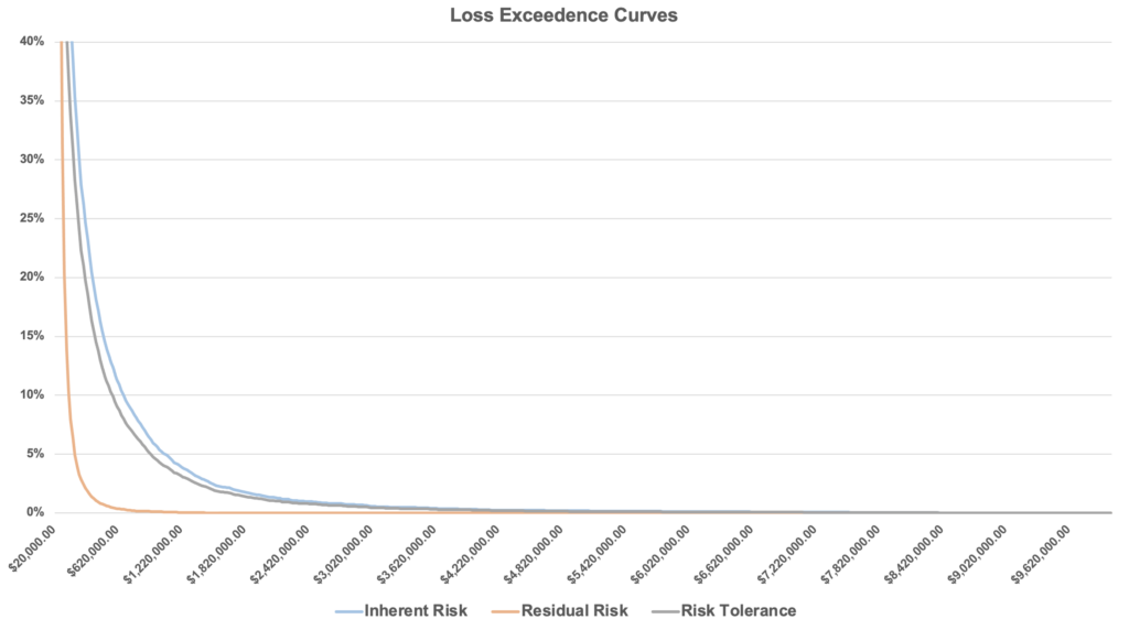
There are actually three exceedance curves in the above graph. The first curve (blue) is inherent risk, which measures current risk. What is the current risk by not purchasing this tool/service?
Residual risk (orange) represents the risk that remains after purchasing the tool/service.
Finally, the risk tolerance curve is defined by someone in the organization with the authority to decide the amount of risk shouldered.
What’s significant is that the residual risk curve is lower than the inherent risk because it means buying the tool reduces risk. Accordingly, if the residual risk curve is below the risk tolerance curve, it signifies that the company is taking on less risk than its maximum.
Yes, It’s Still a Guess, But..
There is never going to be an absolutely correct answer because it’s risk, and risk represents uncertainty. No one knows what will happen in the future. Getting an exact probability for whether you will be breached next year is always going to be a guess.
Using these methods and models, a team can improve guesswork and make more accurate estimations without adding uncertainty. By constraining inputs to educated ranges and replicating thousands of times, these models make your guesses better.
Listen
Catch the concept developer for this article, Sara Anstey, in her interview on the Reimagining Cyber podcast where she talks about her role as Data Analytics Manager at Novacoast: